
Scenario
As the name suggests, there are two different species present in this model: prey and predator. The prey species has a steady inflow of resources (e.g. by eating plants, whose population dynamics are not represented in this model). The predator species feeds on the prey. Both species expend resources to uphold their structure (“living costs”) and to reproduce, which happens in an asexual manner (i.e. individuals can reproduce without a mate).
The interaction consists of the predator moving on the grid and looking for prey in its neighborhood. Upon making contact, it consumes the prey. The prey may flee with a certain probability.
Implementation
This is modelled using a cellular automaton (CA). Each cell of the CA has four possible states:
- Empty
- Inhabited by a prey
- Inhabited by a predator
- Inhabited by both a prey and a predator
No two individuals of the same species can be on the same cell at the same time. Consequently, each cell contains a variable for each species, in which the resource level of the respective individual is stored. The interaction is calculated for each time step and consists of four sequentially applied rules:
- Cost: resources of each individual are depleted by the cost of living. Individuals with negative or zero resources die and are hence removed.
- Movement: predators move to a cell populated by prey in their neighborhood, or to an empty cell if there is no prey. Prey that are on a cell together with a predator flee to an empty cell in their neighborhood with a certain probability. If there are several cells in the neigborhood that meet the above condition, one is chosen at random.
- Eating:: prey consume resources and predators eat prey if they are on the same cell.
- Reproduction: if an individual’s resources exceed a certain value and if there is a cell in its neighborhood that is not already populated by an individual of the same species, it reproduces and an individual of the same species is created on the empty cell. 2 resource units are transferred to the offspring.
All cells are updated asynchronously. The order for the cell update is random for rules 2 and 4, to avoid introducing any ordering artefacts. For rules 1 and 3, this is not required.
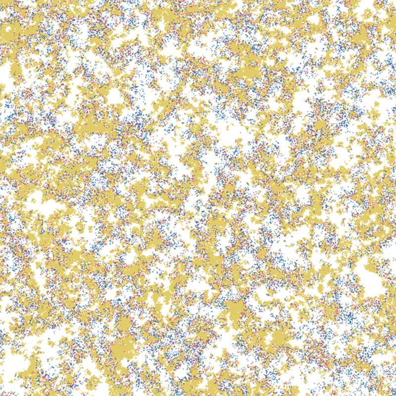
Initialization
Cells are initialized in a random fashion: depending on the probabilities configured by the user, each is initialized in one of the four states. The parameters controlling this are given in the model configuration.